Building Micrograd in Golang

08 Jul, 2024

TLDR - Implementing Micrograd (a scalar-based autograd engine created by Andrej Karpathy) in Golang.

Table of Contents

1. Introduction
2. Basics of Neural Networks
3. Graphs and Autograd
4. The Value Object
5. Building a Neural Network
6. Training the Network

Introduction

This past weekend, I decided to dive into Andrej Karpathy's Zero to Hero course. If you haven't heard about it, it's one of the best ways to learn about building neural networks from first principles. The first video is a spelled out intro to neural networks and backpropogation. This video introduces Micrograd which is small python library that implements backpropogation and a small neural network library.

At Brev.dev (now NVIDIA), our tech stack is primarily written in Go, so I wanted to challenge myself to implement the repo in Golang.

Before we dive in, a few quick notes:

• If you're starting Micrograd in Go (or any other language), don't stress too much about the matplotlib graphing stuff Karpathy does in the video. Just keep a Jupyter Notebook handy for visualizations.
• Do focus on implementing the dot chart. Most languages have bindings for Graphviz. I'd recommend feeding Karpathy's Python dot format, your language's bindings, and your code to Claude 3.5 to get an output. It's super helpful when you're trying to check your implementation of Value and if you've set up the children correctly. My workflow involved writing a Test_Graph function where I'd plug in Value operations and generate a PNG.
• The learning method that worked best for me was: watch Karpathy explain a concept, tinker with the cell, and then try to implement it on my own.

Basics of Neural Networks

At its core, a neural network is just an extremely sophisticated function. It takes inputs, performs some set of operations, and produces outputs. But unlike traditional functions where we explicitly define the rules, neural networks learn these rules from data.

Consider a simple function:

func squareAndAdd(x float64) float64 {
    return x*x + 1
}

This function has a clear, predefined rule. The output will always be the input squared and added. But what if we wanted to create a function that mimics this behavior without knowing the squareAndAdd rule beforehand? That's where neural networks come in.

The Building Blocks: Neurons

The fundamental unit of a neural network is a neuron. In mathematical terms, a neuron performs the following operation:

Here, $x_i$ are inputs, $w_i$ are weights, $b$ is a bias term, and $\sigma$ is an activation function. This is simply a weighted sum followed by some sort of non-linear transformation.

How a Neural Network Learns

A neural network learns to mimic our squareAndAdd function through a process of trial and error, guided by a loss function and optimization.

Let's say we provide some example inputs and outputs:

data := []struct{X, Y float64}{
    {0, 1}, {1, 2}, {2, 5}, {3, 10}
}

A neural network starts with a set of weights and biases. It then:

1. Makes predictions on what the output should be (Forward Pass)
2. Compares predictions to actual outputs using a loss function
3. Adjusts its weights and biases to reduce the loss (Backward Pass)

The loss function quantifies how "wrong" our network is. A common choice for continuous outputs is Mean Squared Error (MSE):

The learning happens in the backward pass. We compute how much each weight and bias contributes to the error and adjust it accordingly using the concept of derivates. This is where the concept of an autograd engine comes in – it automates this process of computing gradients.

Diving into Autograd

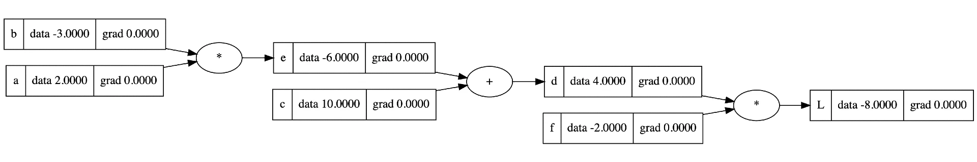
An autograd engine is a system that tracks computations and automatically calculates gradients. It does this by building a computational graph of operations performed on input data, then using this graph to compute gradients efficiently through backpropagation. Here's a toy example from Karpathy's video.

Lets dive a bit deeper into the process

1. Graph Construction: As computations are performed, the engine builds a directed acyclic graph (DAG) where nodes represent operations and edges represent the flow of data.
2. Value and Gradient Tracking: Each node in the graph stores both its computed value and a placeholder for its gradient.
3. Topological Sorting: The graph is sorted in topological order to ensure that gradients are computed in the correct sequence during the backward pass.
4. Gradient Computation: Starting from the output and moving backwards, gradients are computed and accumulated at each node using the chain rule.

At the end of the day, a neural network is simply a very large and complex DAG.

Implementing the Value

The core of micrograd-go is the Value struct. This represents a node on our computational graph and contains the information necessary for calculating the gradients.

The Value struct is contained in the engine.go file.

type Value struct {
    Data     float64
    Label    string
    Grad     float64
    prev     []*Value
    op       string
    Backward func()
}

Here's what each field represents:

• Data: The actual numerical value of this node.
• Label: A string label for debugging and visualization purposes.
• Grad: The gradient of the final output with respect to this value.
• prev: Pointers to the previous Value nodes in the computation graph.
• op: The operation that produced this Value.
• Backward: A function that computes the gradient for this node during backpropagation.

Creating a New Value

We create new Value instances using the NewValue function:

func NewValue(data float64, label string, prev []*Value) *Value {
    return &Value{data, label, 0.0, prev, "", nil}
}

This function initializes a new Value with the given data and label, setting the initial gradient to 0 and leaving the operation and backward function undefined.

Implementing Basic Arithmetic Operations

We start by implementing addition and multiplication (which makes it easy to implement subtraction and division).

func (v *Value) Add(v2 *Value) *Value {
    out := &Value{Data: v.Data + v2.Data, prev: []*Value{v, v2}, op: "+"}
    out.Backward = func() {
        v.Grad += 1.0 * out.Grad
        v2.Grad += 1.0 * out.Grad
    }
    return out
}

func (v *Value) Multiply(v2 *Value) *Value {
    out := &Value{Data: v.Data * v2.Data, prev: []*Value{v, v2}, op: "*"}
    out.Backward = func() {
        v.Grad += out.Grad * v2.Data
        v2.Grad += out.Grad * v.Data
    }
    return out
}

These methods create a new Value representing the result of the operation. They also define the Backward function, which specifies how to compute gradients during backpropagation. The repo contains implementations for a couple other operations including some non-linear transformations.

The Backward Pass

The BackwardPass method is where the magic of automatic differentiation happens:

func (v *Value) BackwardPass() {
    topo := []*Value{}
    visited := map[*Value]bool{}

    topo = buildTopo(v, topo, visited)

    v.Grad = 1.0

    for i := len(topo) - 1; i >= 0; i-- {
        if len(topo[i].prev) != 0 {
            topo[i].Backward()
        }
    }
}

This method does several important things:

1. It builds a topological ordering of the computation graph.
2. It sets the gradient of the final output to 1.0 (we differentiate with respect to the output).
3. It traverses the graph in reverse topological order, calling each node's Backward function to propagate gradients.

The buildTopo function performs a depth-first search to create the topological ordering:

func buildTopo(v *Value, topo []*Value, visited map[*Value]bool) []*Value {
    if !visited[v] {
        visited[v] = true
        for _, prev := range v.prev {
            topo = buildTopo(prev, topo, visited)
        }
        topo = append(topo, v)
    }
    return topo
}

This topological ordering ensures that we compute gradients in the correct order, from the output back to the inputs.

Building a Neural Network

Now that we have our core Value struct implementing automatic differentiation, we can use it to build more some simple neural network components.

Implementing the Neuron Struct

Here's how we define a Neuron struct in our nn.go file:

type Neuron struct {
    Weight []*engine.Value
    Bias   *engine.Value
}

Each neuron has a set of weights (one for each input) and a bias term. We initialize these with random values:

func NewNeuron(nin int) *Neuron {
    var w []*engine.Value
    var b *engine.Value

    for i := 0; i < nin; i++ {
        w = append(w, engine.NewValue(rand.Float64()*2-1, "w", []*engine.Value{}))
    }

    b = engine.NewValue(rand.Float64()*2-1, "b", []*engine.Value{})

    return &Neuron{w, b}
}

The Forward method of a neuron computes its output:

func (n *Neuron) Forward(x []*engine.Value) *engine.Value {
    activation := n.Bias
    for i, input := range x {
        activation = activation.Add(n.Weight[i].Multiply(input))
    }
    return activation.Tanh()
}

This method computes the weighted sum of inputs, adds the bias, and applies the tanh activation function.

Creating Layers

A layer is simply a collection of neurons. We define it as follows:

type Layer struct {
    Neurons []*Neuron
}

func NewLayer(nin int, nout int) *Layer {
    var neurons []*Neuron
    for i := 0; i < nout; i++ {
        n := NewNeuron(nin)
        neurons = append(neurons, n)
    }
    return &Layer{neurons}
}

The Forward method of a layer applies the forward pass to each of its neurons:

func (l *Layer) Forward(x []*engine.Value) []*engine.Value {
    var outputs []*engine.Value
    for i := 0; i < len(l.Neurons); i++ {
        outputs = append(outputs, l.Neurons[i].Forward(x))
    }
    return outputs
}

Implementing the MLP (Multi-Layer Perceptron)

Finally, we can create a multi-layer perceptron by stacking layers:

type MLP struct {
    Layers []*Layer
}

func NewMLP(nin int, nout []int) *MLP {
    var layers []*Layer
    layerSizes := append([]int{nin}, nout...)
    for i := 0; i < len(nout); i++ {
        l := NewLayer(layerSizes[i], layerSizes[i+1])
        layers = append(layers, l)
    }
    return &MLP{layers}
}

The Forward method of the MLP chains the forward passes of its layers:

func (m *MLP) Forward(x []*engine.Value) []*engine.Value {
    for _, layer := range m.Layers {
        new := layer.Forward(x)
        x = new
    }
    return x
}

Implementing the Forward Pass

As we've seen, the forward pass is implemented at each level of our neural network:

1. At the neuron level, it computes the weighted sum of inputs, adds a bias, and applies an activation function.
2. At the layer level, it applies the forward pass to each neuron in the layer.
3. At the MLP level, it chains the forward passes of each layer.

This hierarchical structure allows us to easily compute the output of our entire network for a given input. Moreover, because we're using our Value struct, which tracks the computational graph, we're automatically setting up the network for backpropagation.

Training the Network

Now that we have our neural network components in place, we can focus on the training process. This involves implementing a loss function, creating a training loop, and updating the network parameters based on the computed gradients.

Implementing the Loss Function (MSE)

We'll use Mean Squared Error (MSE) as our loss function. Here's the implementation from the nn.go file:

func MSE(y_pred, y_obs []*engine.Value) *engine.Value {
    if len(y_pred) != len(y_obs) {
        panic("y_pred and y_obs must have the same length")
    }
    sum := engine.NewValue(0.0, "sum", []*engine.Value{})
    for i := 0; i < len(y_obs); i++ {
        diff := y_obs[i].Subtract(y_pred[i])
        squaredDiff := diff.Multiply(diff)
        sum = sum.Add(squaredDiff)
    }

    n := float64(len(y_obs))
    mean := sum.Multiply(engine.NewValue(1/n, "1/n", []*engine.Value{}))
    return mean.AddLabel("MSE")
}

This function computes the average of the squared differences between predicted and observed values. Note how we're using our Value struct operations, which allows the loss computation to be part of the computational graph.

Creating the Training Loop

Now, let's examine the training loop from the train.go file:

func main() {
    // ... (initialization code omitted for brevity)

    mlp := nn.NewMLP(3, []int{4, 4, 1})
    learningRate := 0.01

    for i := 0; i < 500; i++ {
        // Forward pass
        y_pred := make([]*engine.Value, len(x))
        for j, x_i := range x {
            y_pred[j] = mlp.Forward(x_i)[0]
        }

        // Compute loss
        loss := nn.MSE(y_pred, y_obs)

        // Backward pass
        loss.BackwardPass()

        fmt.Printf("Iteration %d: Loss: %.6f\n", i, loss.Data)

        // Optimizer
        for _, p := range mlp.Parameters() {
            p.Data = p.Data - (learningRate * p.Grad)
            p.Grad = 0.0
        }
    }

    // ... (final predictions code omitted for brevity)
}

Let's break down the key components of this training loop:

1. Initialization: We create an MLP with 3 input neurons, two hidden layers of 4 neurons each, and 1 output neuron.

2. Forward Pass: For each training example, we perform a forward pass through the network to get predictions.

3. Loss Computation: We calculate the MSE loss between predictions and observed values.

4. Backward Pass: We call loss.BackwardPass(), which triggers the backpropagation through our computational graph, computing gradients for all parameters.

5. Parameter Update: We update all parameters using a simple gradient descent step.

Updating Parameters Using Gradients

The parameter update step is a critical part of the training process. Let's look at it in more detail:

// Optimizer
for _, p := range mlp.Parameters() {
    p.Data = p.Data - (learningRate * p.Grad)
    p.Grad = 0.0
}

This code iterates over all parameters of the MLP. For each parameter:

1. It updates the parameter value by subtracting the product of the learning rate and the gradient. This is the core of gradient descent: we move the parameter in the opposite direction of the gradient to minimize the loss.

2. It resets the gradient to zero. This is crucial because gradients are accumulated during backpropagation, and we need to start fresh for the next iteration.

The mlp.Parameters() method (from nn.go) collects all trainable parameters:

func (m *MLP) Parameters() []*engine.Value {
    var params []*engine.Value
    for _, layer := range m.Layers {
        params = append(params, layer.Parameters()...)
    }
    return params
}

This method recursively gathers parameters from all layers, which in turn gather parameters from all neurons.

By repeating this process of forward pass, loss computation, backward pass, and parameter update, we gradually adjust the network's parameters to minimize the loss function. Over time, this should lead to improved predictions on our training data.

Conclusion

There's no better way to learn something new than implementing it yourself in a different language. That certainly rang true for this. However, there were some challenges while implementing this in go.

The first one was a lack of notebook support. Jupyter NBs seem to be a very polarizing topic in the community but theres no doubt they're one of the best tools for teaching and iterating quickly on something new. To simulate this in Go, I could only write tests as I went through the tutorial.

The lack of operator overloading was also a cause for some discomfort. The original micrograd library is extremely short due to the Value class being able to overload addition, subtraction, etc. In Go, I had to implement each method myself increasing the length of the library.

The entire codebase can be found in this repo. Thanks for reading :)